Good morning, sunshine! 😊 A great party last night? Unfortunately, you’ve lost your phone: it seems one of your “friends” has left with it. In this lesson, we’ll have to find out who.

But luckily, your phone is still logging data! You can catch the culprit using time series analysis!

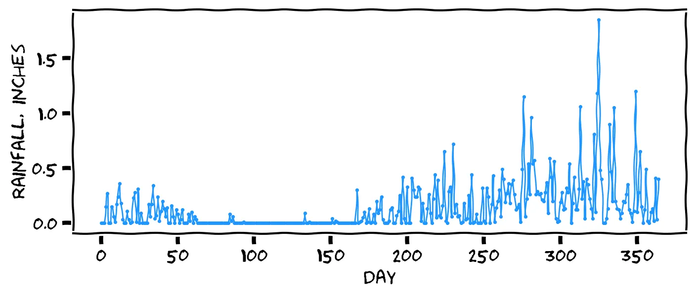
You recently learned about time series in your day job at $\text{C}\undergroup{\text{ongo}}\text{.com}$. Every night, to keep the package deliveries running smoothly, the server calculates the best delivery routes for the next day. To calculate the best routes, it needs a rainfall prediction. If the prediction is wrong, mopeds get stuck on muddy roads, and packages are delayed.

On average, it rains $0.14$ inches per day in your area of the Congo. But on the week you arrived at the company, it rained over an inch every day from Monday to Friday. Judging from this week of rain, we should say that Saturday’s rain will probably be ...

Before you joined $\text{C}\undergroup{\text{ongo}}\text{.com}$, your colleague Eva had written the first rainfall prediction program. No matter what, Eva’s program predicts that tomorrow’s rainfall will be $0.14$ inches. After five days of rain, what did Eva’s program predict for Saturday’s rainfall?

But lo and behold, on Saturday it poured down again. The route planner was chaos, and you saw a cheap way to make your mark on the company. What if, instead of predicting that “tomorrow’s rainfall will be the average”, we instead predicted that “tomorrow’s rainfall will be the same as today’s measured rainfall”? How do you think this new method would compare to Eva’s?

You open up Eva’s file predict_rainfall.py and find:

Here, predict is a Python function. You give it tomorrow’s date t, and it returns the predicted rainfall in inches. Eva’s function always returns 0.14.

You first change the program to fetch the true rainfall measurements from the local weather API. You put this in an array M, where M[t] is the true rainfall on date t.

Now you need to edit the predict function to say: “tomorrow’s rainfall will probably be the same as today’s measured rainfall.” Given date t, what should your function return?

You pull an all-nighter to make this change, then go to bed. But you wake up to an unpleasant surprise: Eva is reviewing your change, and she’s annoyed that you’ve replaced her code!

So you set about to prove that your model is better, using Science 🔬. You look up the last year of rainfall in Kinshasa, and draw up a table:

Here, Eva[t] and You[t] are predictions for day t. Judging from the days shown, which program is better?

As always, an excellent question! Your boss says the “better” model is the one that “makes $\text{C}\undergroup{\text{ongo}}\text{.com}$ the most money”. However, this is rather hard to determine, so data scientists often use something called mean squared error, or MSE.

For each prediction, you take the difference between the prediction and the true measurement, then square the difference. This gives you a positive number, called squared error. What was Eva’s squared error on Feb 16th?

You need to run this calculation for every day in the last 12 months. The “best” model is then the one with the lowest mean squared error (MSE).

Fine, I’ll do it. When we look at twelve months of rainfall, your model’s MSE is $0.063$, and Eva’s MSE is $0.049$. So, which is better?

It seems that, although the weather has some tendency to follow yesterday, it has a stronger tendency to “regress to the mean”.

You can’t let it go: Eva’s model just looks naïve, and it feels like yours should work better. Eventually, after some bickering, your boss has a word with you both: “Come on, folks. What if we just averaged your two models?”:

Indeed! Surely we have to resolve this argument with science, not with politics! But to prove your point, you find the mean squared error for your manager’s suggestion, too.

To your horror, you find that the compromise model works better than either your model or Eva’s, with an MSE of just $0.044$! This is an example of the “ensemble” phenomenon: when you combine a diverse set of models, the result is often better than any of the individuals. This is particularly true when the set of models is “diverse”, because they tend to cancel out each other’s biases.

After this discovery, you and Eva decide to end your rivalry (“We were both right!”). Visiting the dusty corporate library, you find The Old Time-Series Textbook, where you discover that you’ve re-invented something called the “auto-regressive model”, or AR model.

You’ve been working in Python, but all the textbooks use math notation. In time series notation, the prediction is written $X_t$, the true value measurement M[t] can be written as $M_t$, and the error is written ${ϵ}_t=M_t-X_t$. The Textbook says an AR model looks like:

The numbers $\mu$ (“mu”) and $\varphi$ (“phi”) are called parameters. If you write the above “compromise” model in this notation, what are its parameters?

Your rainfall model only looks as far back as the previous day. This is called an $\text{AR}(1)$ model. But in its general form, an $\text{AR}(p)$ model looks back at the past $p$ days:

The hyperparameter $p$ is the number of days to look back. So an $\text{AR}(p=1)$ model has $p+1$ parameters: one $\mu$ parameter, and then a ${\varphi }_i$ parameter for each day $i$. Think back to Eva’s simple model, $X_t=0.14$. What is the value of $p$ for Eva’s model?

Eva’s was an $\text{AR}(p=0)$ model, with just one parameter, $\mu =0.14$. It doesn’t look back at any previous days.

Forget the phone, we’ll come back to it! Anyway, one night, you woke up in a sweat with an idea. Eva’s simple model of “always estimate the average” turned out to be decent. But it had one weakness: an overly static idea of “the average”. What if the average changes over time? Say, due to climate change? And so what if our model could adjust its estimate of “the average” in response to new data?

Here’s an example. On Sunday, you predicted that on Monday it would rain the average: $0.14$ inches. But on Monday, it actually rained $0.24$ inches. What went wrong? Perhaps our estimated average, $0.14$, is ...

We want to continue with our strategy of just “estimate the average”, but revise our estimate of the average, closer to $0.24$. We don’t want to move it all the way to $0.24$: this will just result in your first model, and we’ve seen already that this performed worse. But we could move it, say, $10\%$ closer to $0.24$.

If you did this, what should you update your average to?

In general, we can move $10\%$ closer to the measurement using a weighted average:

Since we always predict the average, $X_t$ stands for our prediction and our estimate of the average, and the above equation is used both for updating our average, and for making a new prediction.

After running this new model on a year of rainfall data, you find that it’s the best model yet, with an MSE of just $0.037$!

According to The Textbook, you’ve just invented the “moving average” (MA) model. It’s usually combined with the AR model to create the ARMA model. The simplest ARMA model is $\text{ARMA}(p=1,q=1)$, which can be written as:

This adds a new term, $\theta {ϵ}_{t-1}$. As before, ${ϵ}_t=M_t-X_t$ is the error for day $t$. The new parameter $\theta$ says how much to move the average.

To move our average $10\%$ closer to the measurement, we’ll set $\mu =0$ and $\varphi =1$. But what should our $\theta$ be?

In its general form, the $\text{ARMA}(p,q)$ model looks back at the past $p$ measurements, and the last $q$ errors:

Now for a word of warning. Suppose you wanted to say: “tomorrow’s rainfall will be the average of the previous 31 days.” What kind of model would you express this with?

Snap back to your missing phone. You crack open your laptop, and find that your phone is still broadcasting data! Surely you can use this to discover the culprit. One of the data streams is from the accelerometer. The accelerometer tells you the device’s acceleration (e.g. gravity, used for automatic screen rotation). This can be formed into a time series, with the magnitude of acceleration over time. And when you’re walking, which apparently the thief is doing right now, it looks like this:

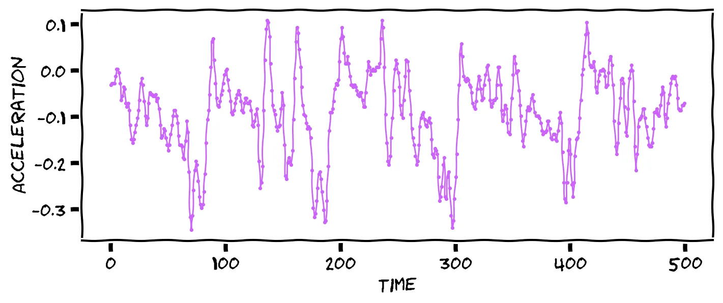
That wouldn’t hold up in court, my friend. What did Jacques do to you, anyway? No, we need to be more systematic. Luckily, you have samples of the accelerometer data for the 32 friends who were at your party:

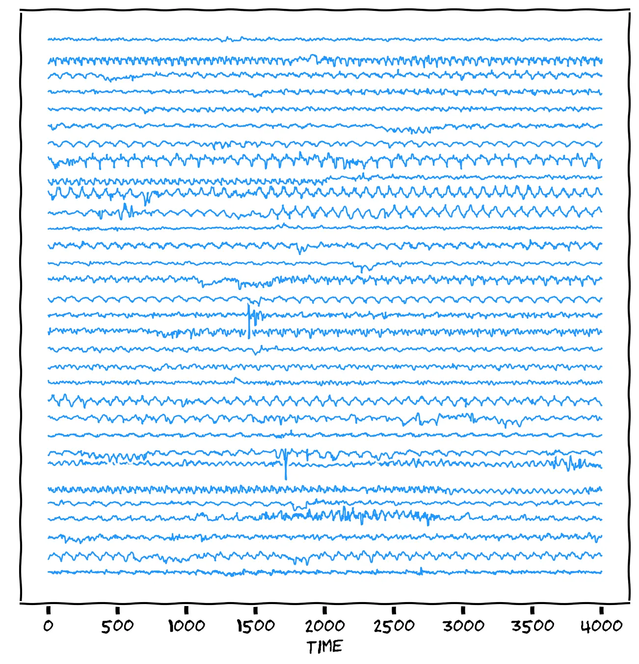
It’s amazing how much data $\text{C}\undergroup{\text{ongo}}\text{.com}$ collects! 🤭 Best not speak any further of it. The question is, which of those friends generated the thief’s data? Notice that each time series repeats as the person walks, but each walk has a different shape. Your walk has enough information to determine who you are!! So, compare the thief’s accelerometer chart to each friend’s accelerometer chart. Which one is the thief most similar to?

But how can we get the computer to see the different shapes, amidst all the random vibrations and noise? Well, we can use an ARMA model to summarize each walk! Then, instead of comparing messy charts with thousands of data points, we’d just be comparing a few numbers.

So far, you have been finding model parameters by trial and error. This process of finding the best parameters is called fitting.

You really don’t want to fit all 32 models by hand. Luckily, data scientists have a way to make the computer to do the hard work: automatic function minimization. Minimization is the most powerful dark magic in all of data science, and in your career, you will use it for everything.

In this lesson, we’ll use the minimize function from scipy. You give it a function, and it tries to find the input that minimizes the output. Consider the function $f(x)=(x-2{)}^2$. Use your brain: what value of $x$ results in a minimum value of $f(x)$?

Perhaps you solved that one by trial-and-error, or some clever calculus. But we can get the computer to do it for us, with no brain required! First, we write the function in Python:

Then we call minimize(f, 42). The value 42 is an initial guess at the minimum, and any other value will work here. Within a blink of an eye, it will return the minimum, 1.99999999.

No, it didn’t quite return $2$, but 1.99999999 is close enough for jazz. Basically, minimize uses trial-and-error, and stops when it finds a “good enough” answer.

The minimize function also works on functions with multiple parameters. Here’s an example of minimizing $d(x,y)=x^2+y^2$:

The function $d(x,y)$ measures the (squared) distance of a point $(x,y)$ from the origin. So what input would minimize this function?

The closest point to the origin is the origin itself, $(0,0)$. Therefore, minimize returns the origin: [0.000002, -0.000001].

Earlier, we were trying to find the best parameters to minimize a number called “mean squared error”. You were using trial and error. But we can do it automatically using minimize!

Let’s see how to do this to fit an $\text{ARMA}(1,1)$ model to the thief’s time series. First, we write a Python function for the model:

Then we write a function MSE which, given candidate parameters mu, phi and theta, runs the model on the thief timeseries, and returns the mean squared error:

Which function should we run minimize on?

So we run minimize on the MSE function, with an arbitrary guess at the parameters:

Quickly, it tells us the parameters that minimize the mean squared error: $\mu =0$, $\varphi =0.91$, and $\theta =0.73$. We’ve got the thief’s walking fingerprint! Now we just need to find a match in the database! 🕵️

Earlier, we were using the model parameters to predict the future of the time series. But another way we can use the learned parameters is as a kind of summary, signature, or fingerprint. Then we can compare one time series’ signature to the signatures of time series that we have recorded before. This is called time series classification.

Sadly, your phone doesn’t log GPS. But that sure is convenient for me teaching you time series! So for each person’s data you get their fingerprint $F=(\mu ,\varphi ,\theta )$. You can imagine each person’s fingerprint $F$ as a point in 3D space. Here’s a 3D plot of the parameters for each friend’s fingerprint:

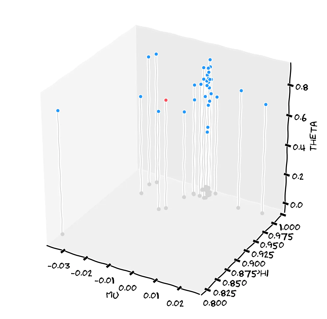
The point $F_{\text{thief}}=(0,0.91,0.73)$ is plotted above in $\text{red}$. How can you determine which friend’s fingerprint it most closely matches? One way is Euclidean distance: “which known point is it closest to in 3D space?” (We just have to scale the axes a bit. Notice the points are clustered closely around $\mu =0$, but $\theta$ varies much more.)

Okay, here are your friends’ distances to the thief fingerprint:

Yes, it does seem that it was your colleague, Jacques. Well done. As you can see, the computer is quite sure that it was Jacques: his distance to the thief ($0.36$) is well below every other friend’s distance. On this basis, $\text{C}\undergroup{\text{ongo}}\text{.com}$ suspended Jacques pending an investigation.

Whenever you have a problem, try expressing it as a function that minimize can solve. You’d be surprised how many problems can be solved this way! Even problems like “create an AI that draws amazing illustrations from a text prompt” are essentially solved by running minimize on a sophisticated function.

You probably noticed the privacy implications of today’s analysis. It’s concerning, although most companies don’t actually track your accelerometer. And there are many less creepy applications of time series analysis. Try applying it to your spending habits; I bet you’ll see interesting trends that you can use to predict your future spending.

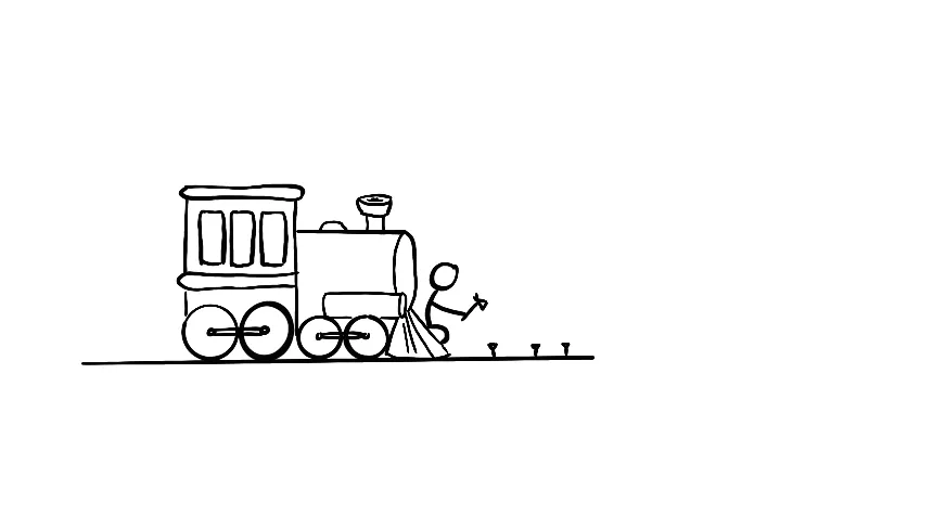
Just a word of warning: there are many time series that are extremely hard to predict and can be frustrating if you’re not prepared. It sometimes feels like time series prediction is like laying down the tracks while on the front of a speeding train.

⭐ To play with the code and data yourself, the notebook is here. Enjoy!

⭐ For an ARMA model to work best, the time series should be stationary (that is, constant mean and variance). And it should not be seasonal (that is, it should not look like that bane of retail workers, "All I Want For Christmas Is You"). To model more challenging series, there are many ARMA variants (see "The ARMA alphabet soup"), as well as completely different ways of modeling time series.

⭐ We chose $\text{ARMA}(p=1,q=1)$ here. You might be tempted to use bigger models like $\text{ARMA}(10,10)$, but this runs the risk of overfitting. Formulas like AIC can help with this tradeoff.

⭐ We fitted the model by minimizing squared error. There are other ways to fit a model, such as maximum likelihood estimation. For a pre-packaged solution, see ARIMA.fitfrom the statsmodels package.

⭐ The minimize function worked well for our functions above. But minimization is a gnarly problem: it’s not guaranteed to find a global minimum, or even a local minimum. It can get stuck, or fly off to infinity, or take longer to finish than the lifetime of the universe.