Ahh, another day working at $\text{C}\undergroup{\text{ongo}}\text{.com}$, the world’s largest online marketplace. This morning, your boss is complaining: lots of users’ product searches have no results. Here are some books on the warehouse shelves:

Grease, Axel. The Complete Idiot’s Guide to Auto Repair. 3rd ed.

Shaft, Camilla. Truckin’ Hell: An Intro to Pickup Upkeep. 2019.

Stands, Jack. Truckers’ Secret Handbook. Revised ed.

...

And yet, if you search for “beginner truck maintenance” – nada. As the resident data scientist, you’ve been tasked with fixing the problem. Here’s the current search algorithm:

Why does the search for beginner truck maintenance return no results?

The current search is doing pure keyword search: it demands that the description contains all the word maintenance, but what if it instead contains synonyms like repair or upkeep?

We don’t just need a keyword search; we need a semantic search. Which of these would be most useful to build a simple semantic search engine?

Unfortunately, the Merriam-Webster is hopelessly out of date, and $\text{C}\undergroup{\text{ongo}}\text{.com}$ has books in 1,000+ languages on every conceivable topic. No, to build our semantic search, we first need to build our own thesaurus.

Indeed, it seems hard to get a computer to measure the meaning of a given word. But perhaps we can instead get the computer to measure whether two given words have similar meaning.

Let’s play a game. I’ve picked two secret words $W_1$ and $W_2$. Your job is to guess whether ${\mathbf{W}}_1$ and ${\mathbf{W}}_2$ have the same meaning. To help make your guess, you can choose just one of the following clues:

To see how this works, we’ll work with this 1GB sample of text from Wikipedia. Data scientists call big collections like this a corpus. In this corpus:

Ten words that often follow $W_1$ are again, airing, construction, operation, play, playing, production, until, work, and working.

Ten words that often follow $W_2$ are again, date, off, out, playing, point, program, until, up, and working.

Now, do you think ${\mathbf{W}}_1$ and ${\mathbf{W}}_2$ are close in meaning?

It seems reasonable to say: if two words are close in meaning, it causes them to have similar following-words. But does this work in reverse? If two words have similar context-words, does that cause them to be close in meaning?

Here’s a thought experiment. Suppose you start a new job. Your co-workers keep using the strange word grond. “Work gronds at 9am. When it finishes, we’ll grond partying.” Over time, you discover that the word grondhas exactly the same distribution of context-words as the word start. Does this mean the word grond means the same as the word start?

There’s evidence that children acquire much of their vocabulary using this method. According to the distributional hypothesis, the list of words surrounding begin is a sort of “fingerprint” of the word begin. A fingerprint that the computer can measure, and perhaps acquire language like children do!

Let’s see how far the distributional hypothesis goes, by playing the word-guessing game once more. I’ve got two new words, $W_3$ and $W_4$.

Ten words often following $W_3$ are 1960s, 1970s, 1980s, 1990s, 19th, 2000s, 20th, days, medieval, and years.

Ten words often following $W_4$ are 18th, 1940s, 1950s, 1960s, 1970s, 1980s, 1990s, 19th, cretaceous, and night.

Do you think ${\mathbf{W}}_3$ and ${\mathbf{W}}_4$ are close in meaning?

We commonly say antonyms are “opposite in meaning”. Yet they share many concepts, and therefore have similar word-contexts. For example, the words early and late share concepts like time, comparisons, and events, and therefore include similar following-words, like 1960s.

So our “word fingerprint” idea is not doomed. It’s just that these fingerprints don’t quite measure synonymousness. They instead measure something more like number of shared concepts. But that’s exactly what we want for our task of finding relevant sentences in a long document!

To build our thesaurus, we’ll first take our big Wikipedia text corpus, and count up which words follow each other. We end up with a big table like this:

We’ve considered the most frequent $10000$ words in the corpus. The table above is a sample from that giant table. It shows four current words, truck, car, build, and manufacture, and two following words, the and is. How many times in the corpus is the word truck followed by the word is?

Above, we said that a word’s “fingerprint” is a list of words that commonly follow it. In the full table, how big is one word’s fingerprint?

That’s pretty big! To keep things manageable for now, let’s just consider two of those following-words, the and is. What is the word fingerprint of the word truck?

Suppose we’re searching in a document for words related to truck. Use your intuition: which of the following words is most related to the word truck?

Let’s see if we can measure that. How could we measure how related any two words are, as a number?

First, some terminology. A vector is a list of numbers. A word fingerprint like [86, 70] is an example of a vector. When we use the word “vector”, it’s usually because we’re visualizing the number-list as the coordinates of a point in space. For example, we can visualize our word fingerprints as points in a 2D space:

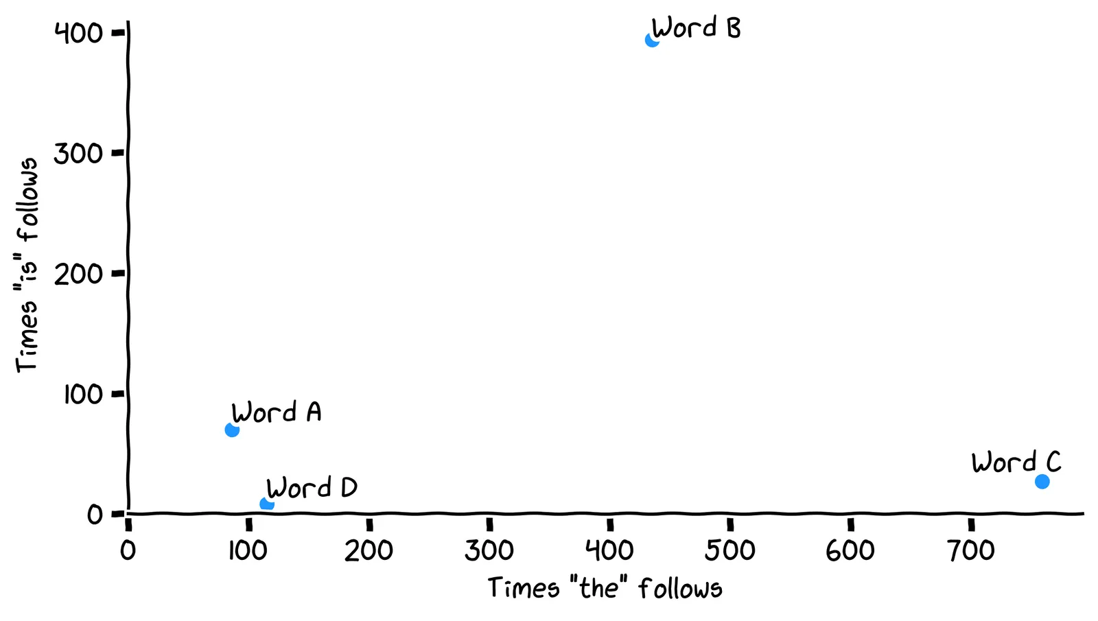
These words are embedded in a 2D space. For this reason, word vectors are usually called embeddings.

Consider embedding C in the plot. Which word does C represent?

A key value of thinking about points in space instead of lists of numbers is that we can intuitively measure distances between points. Here’s Euclid’s formula for measuring the distance between two points in 2D space:

We can use the Euclidean distance formula to find the word with the closest embedding to truck. We’re effectively measuring the lengths of these lines:

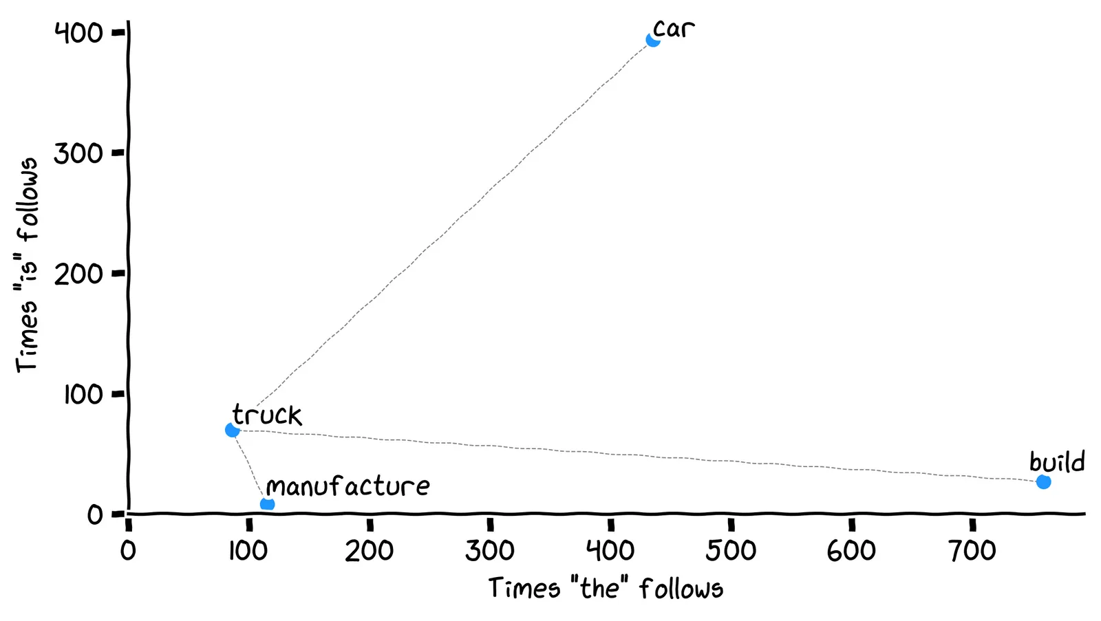
Using this formula, which word embedding is closest to the word truck?

Earlier, we said the closest word to truck should be car. But our distance formula says the closest word embedding is manufacture. Our algorithm is not aligned with our desires.

To “fix” this, which of the following could we change?

Either of these can work! Later we’ll see a solution that changes how we measure distance. But first, let’s see a solution that changes the points of the words on the plot.

What does our space of the vs. is actually represent? Suppose I pick a new word $W_5$, and show you its word vector, $[c_{the},c_{is}]=[13,123]$. What does this vector tell you about the word ${\mathbf{W}}_5$?

The word is commonly follows nouns, as in “the truck is red”. The word the commonly follows verbs, as in “manufacture the truck”. The unknown word is mostly followed by is, so it’s probably a noun. It turns out our plot is mostly a plot of $\text{nouns}$ vs. $\text{verbs}$:

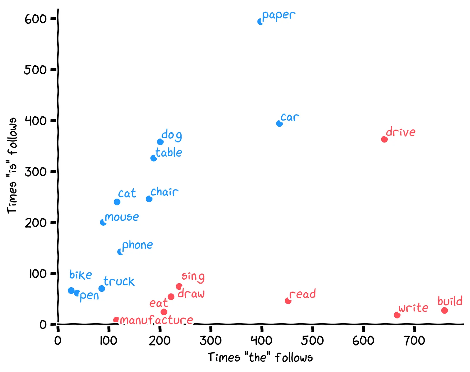
Let’s make this more precise. Say there’s some word embedding $[c_{the},c_{is}]$. Which of the following values would be most helpful to determine whether that word is a noun?

The ratio $\frac{c_{is}}{c_{the}}$ is the most helpful. Nouns will have a high value, significantly above $1.0$.

That ratio $\frac{c_{is}}{c_{the}}$ is the slope of the line from the origin to the point, which we can visualize like this:

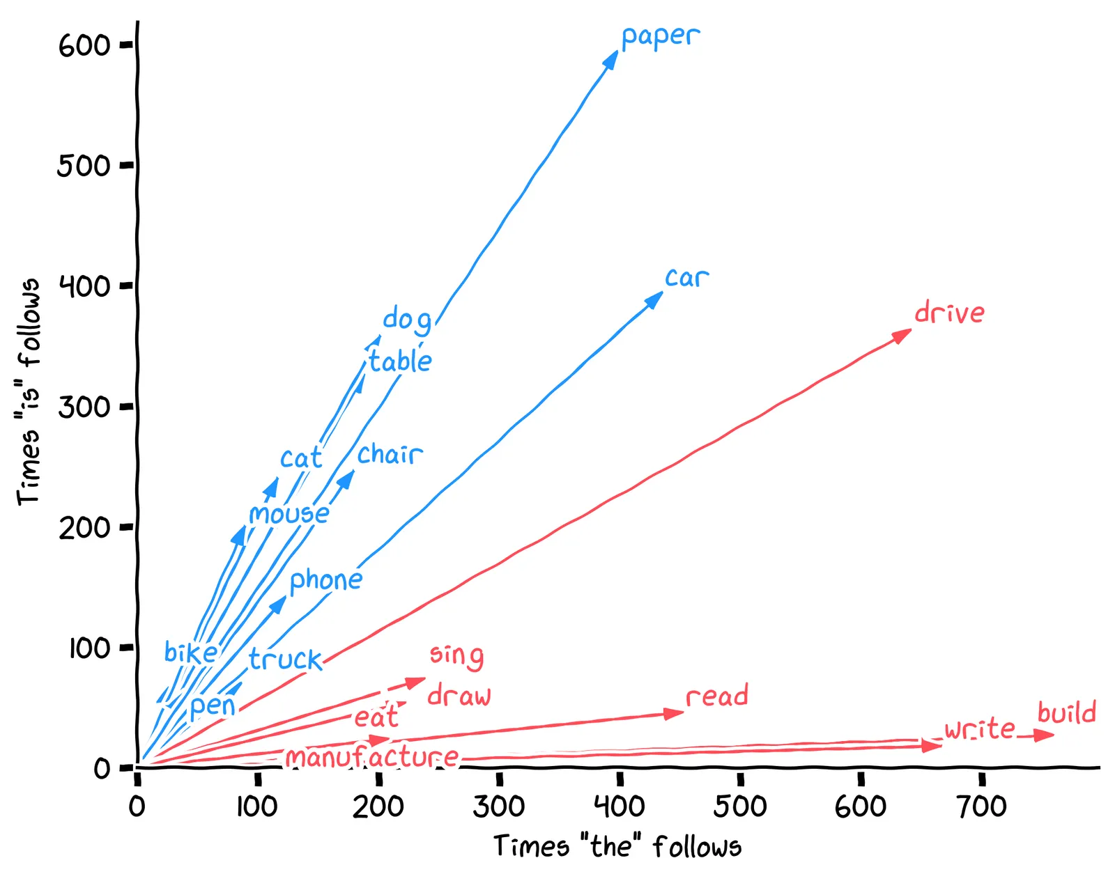
Above, instead of plotting each word as a point, each word is shown as an arrow. This is yet another meaning of the word vector – an arrow that has two things:

A direction: where it “points”.

A magnitude: how long it is.

Given a word vector in our 2D space, the direction of that vector measures the word’s noun-ness. But what does its magnitude measure?

So, when we looked for the closest word to truck, why did we get manufacture rather than car?

For our purposes, we don’t care about word usage frequency. One way we can fix this is to set all magnitudes to $1$. This is called normalization, and it looks like this:

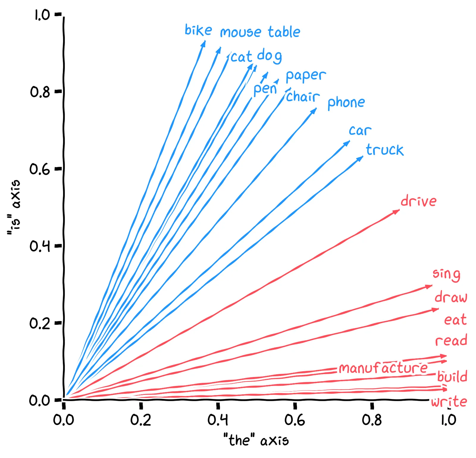
Earlier, when searching words related to truck, the Euclidean distance gave us the word manufacture. After we’ve normalized the vectors, what’s the closest word to truck, using the Euclidean distance?

We’ve made good progress!

Notice how all the arrow-heads of the normalized vectors lie on the unit circle. There’s a natural way to talk about the position of a point on a circle: the angle. Let’s measure the angle between the word truck and each of the other words.

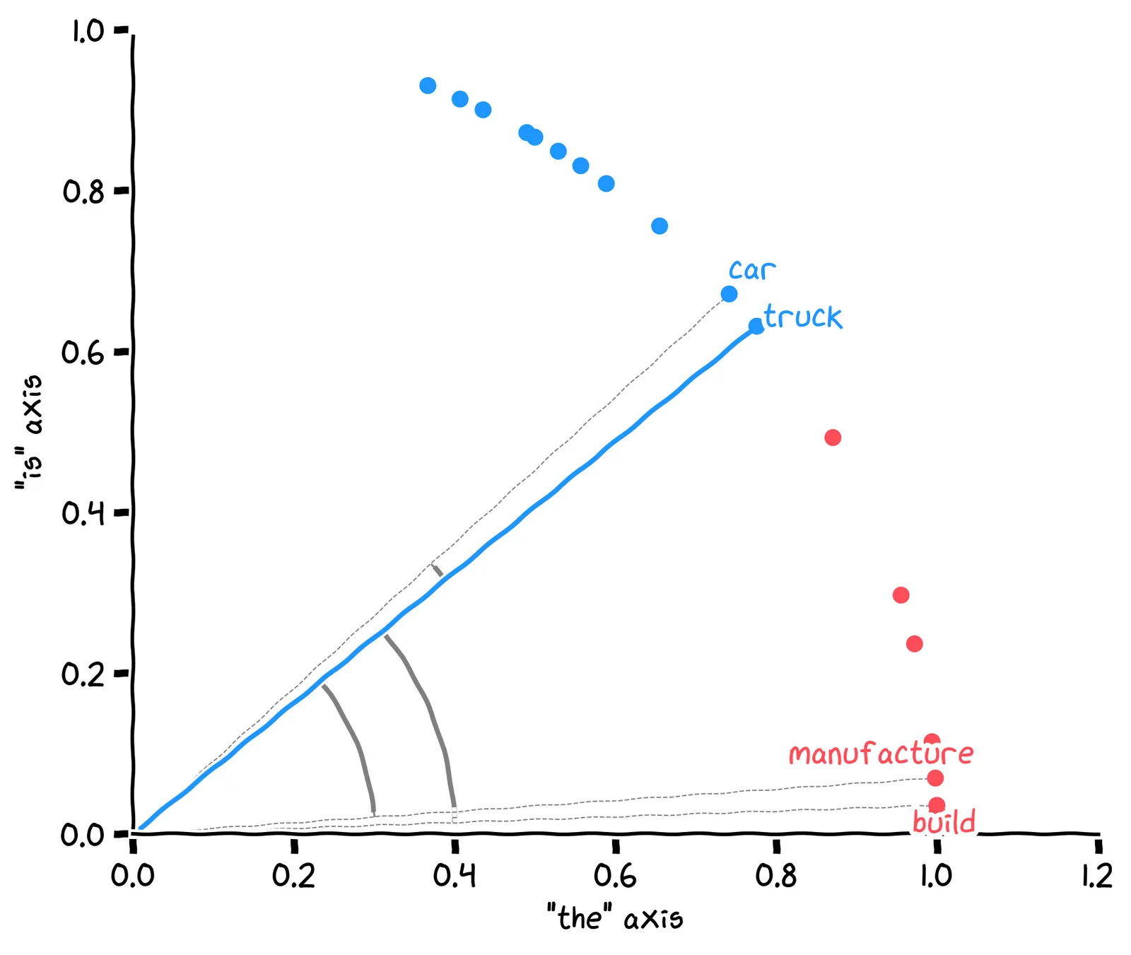
Which word has the closest angle to truck?

Earlier, we saw the Euclidean distance. We’ve found a different kind of distance: interpret the points as vectors, then take the angle between them. This is called the angular distance between two vectors. In our plot of the vs is, what is the largest possible angular distance between two word vectors?

This one is tricky! If the vectors could point in any direction, the largest possible angular distance is $180°$. But all the values in our word vectors are positive counts, so they all point up and to the right. So the largest possible angular distance is only $90°$.

In data science, we don’t often use the angular distance. Instead, we use something called called cosine similarity, written as $S(\vec{a},\vec{b})$. This is the cosine of the angle between the two vectors.

The cosine similarity between two normalized vectors has a formula that’s easy to calculate, called the dot product:

Suppose the normalized vector for the word phone is $\vec{p}=[0.6,0.8]$. What is $\mathbf{S}(\vec{\mathbf{p}},\vec{\mathbf{p}})$, i.e., the cosine similarity between $\vec{\mathbf{p}}$ and itself? (Hint: $\cos (0°)=1$.)

It’s no coincidence that this is $1$. If two vectors point in the same direction, their cosine similarity is $1$. If they point in opposite directions, their cosine similarity is $-1$. And if they are orthogonal, their cosine similarity is $0$. Which of the following has the largest value?

The vector for truck points in the same direction as itself, so the cosine similarity is $1$. The vector for car points in a slightly different direction, so the cosine similarity is a little less: $0.998$.

As a brief interlude, here’s a word puzzle: actor - man + woman ≈ ?

Considered purely as a word puzzle, the answer is actress.

But it turns out that, when we use our full $10,000$-dimensional word vector, this crazy arithmetic actually works! When replacing the words with their word vectors, and doing the arithmetic, we get a vector which is very close to the vector for actress.

Specifically, we’re using vector addition, which is defined as:

Try it yourself: what is $[-1,2]+[1,3]$?

Here’s another: spider - eight + six ≈ ?

Why, it’s ant of course! By the logic of word vectors, an ant is a six-legged spider.

Alright, let’s get back to it. We’d found a way to improve on keyword search: use our word vectors to search for words similar to the query words, then include those in our keyword search.

That’s a valid approach, but let’s go all-in on vectors! You’ve seen that we can encode words as vectors. But, considering our new skill of adding vectors, what else could we encode as vectors?

All of these are possible! You can encode almost anything as a vector! For our purposes, it will be useful to encode sentences and queries. Then we could find the most relevant sentences to our query using the same technology we’ve developed above: cosine similarity between a query vector and a product vector.

But how can we get a vector for a sentence or for the query? One way is just to add together all the word vectors in the sentence. Consider the following two sentences:

Will these sentences get different sentence vectors?

Because addition is commutative, these sentences will get the same sentence vector. Despite this naïve approach, addition can give us a useful summary of a text! Using this technique, we end up with this search engine algorithm:

In this chapter, we built a semantic search engine. Our goal was to find products that are most similar to a query string. We did that by converting all the text to vectors, called embeddings. To find word embeddings, we started with a large corpus, and characterized each word by the distribution of words that follow it. To find embeddings for queries and products, we just added up all their word vectors. To compare those vectors, we settled on normalization plus cosine similarity.

The approach we took here is called word2vec. It’s a classic algorithm for getting word vectors.

To build the vector for a word, we considered just the immediately following words in the corpus. But word2vec considers more “context words”. For example, the two words after the current word, and the two words before it.

We built word vectors with 10,000 dimensions. Real word embeddings are typically smaller, perhaps ~300 dimensions. This can be achieved by dimensionality reduction. word2vec uses a neural network for this, although there are many other methods.

To get sentence embeddings, we just added up the words’ embeddings. This doesn’t allow words to change their meaning based on context. We could have used an “attention” mechanism for this.