One of the greatest pleasures in life is a cool glass of lemonade after a hot day laboring over your keyboard. You’ve spent the afternoon anticipating this evening’s party. Deserving a break, you meander over to the fridge.

To your utmost horror, you find that you drank the last of the lemonade yesterday. Everyone’s coming to your party this evening — but now all you have in the fridge is water, sugar, and whole lemons. And the worst thing: you’ve forgotten the ratio of ingredients! 😲

Not so fast! As an intrepid data scientist, you must design a scientific test which will determine the perfect ratio of water, sugar, and lemons!

You rack your brain ... it was seven cups total, and one cup of lemon juice ... but was it one or two cups of sugar? We’ll call these candidates Recipe $\mathbf{A}$ and Recipe $\mathbf{B}$:

Recipe $\mathbf{A}$: 1 cup lemon juice, 1 cup sugar, and 5 cups of water.

Recipe $\mathbf{B}$: 1 cup lemon juice, 2 cups sugar, and 4 cups of water.

Your job is to discover which of these is best, using an A/B test.

A great question! To answer that, let’s look at a more traditional A/B test.

By day, you work as a data scientist for a large shopping website named after a massive rainforest. $\text{C}\undergroup{\text{ongo}}\text{.com}$. Your website sells tons of goods everyday. However, you believe changes to the product page can increase sales, and profits, even further.

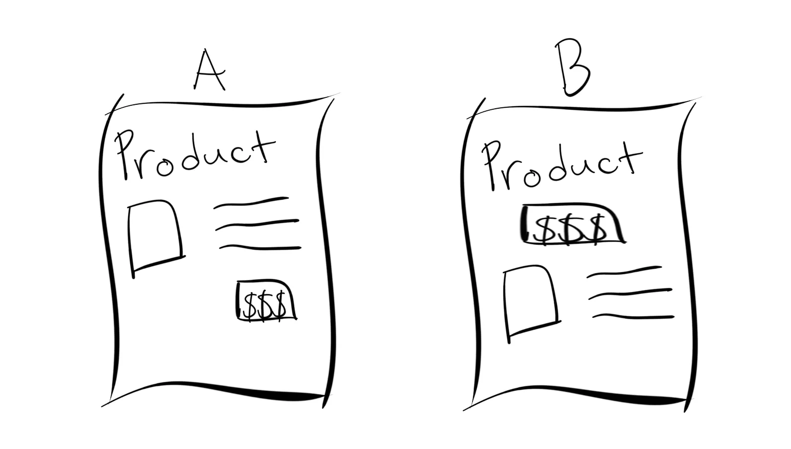
Our current page, shown here as Page $\mathbf{B}$, has the Buy Button (shown here with the $$$ box) before the information about what we are selling. But customers might be better informed, and then end up buying our product, if the button came after the product’s information. That’s shown here as Page $\mathbf{A}$.

We like money, so the “best” page here is the one that gets the most sales. Which page do you think we should use?

A/B testing is a way to test our hypothesis and determine for sure which product page is best. There are many ways to run an A/B test, and they can get very complicated!

Indeed, as an everyday data scientist, your toolkit looks different. So let’s explore the simplest type of A/B test, before taking a peek at more complicated versions.

Continuing with the product page example, you get the go ahead from management to run your test. You work with engineering to build a system that routes people to one of the two pages, randomly, based on a coin flip.

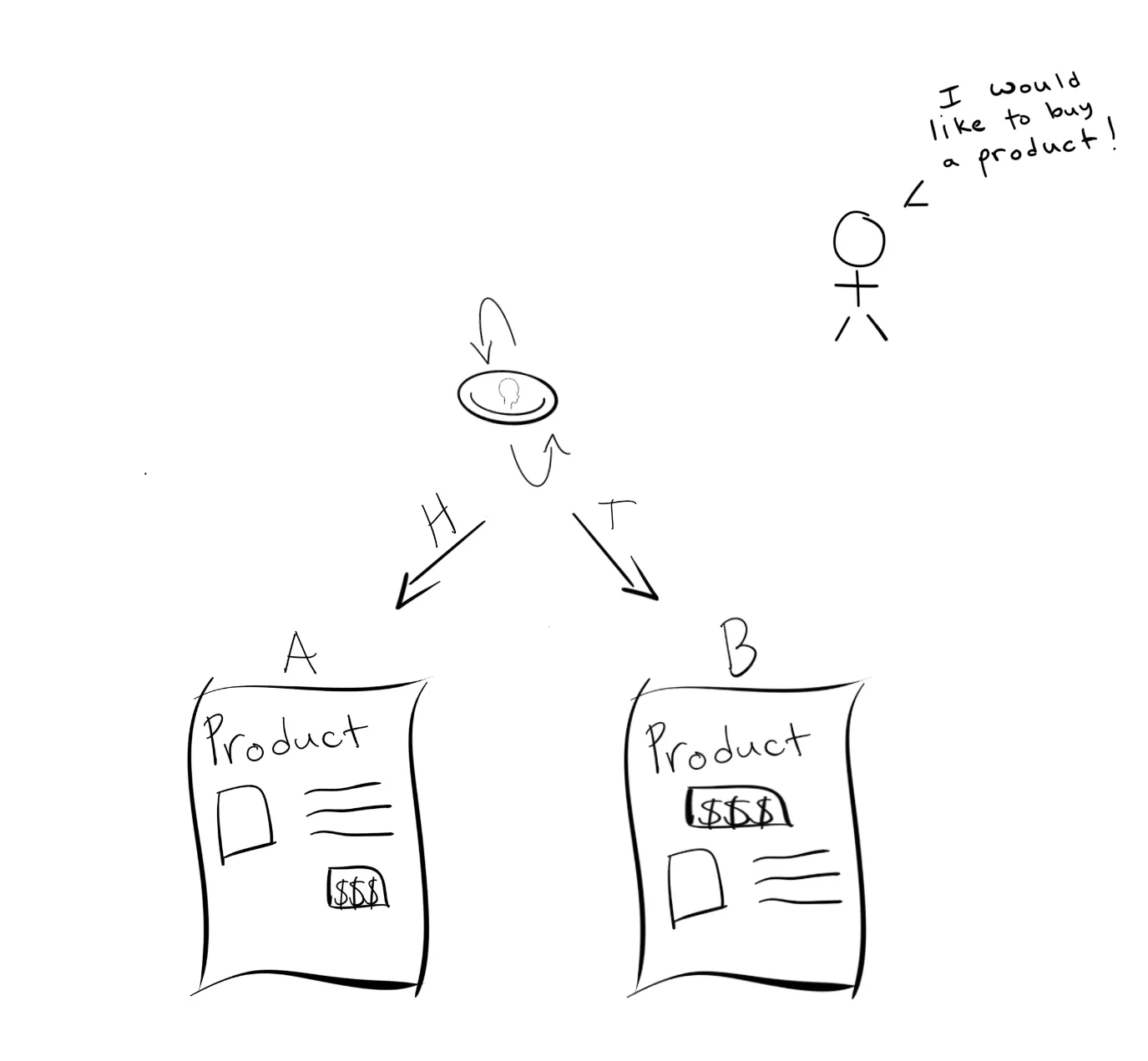
After a while, the data looks like this:

In the lines above, a $1$ means that a customer was directed to the page, and then bought the item. A $0$ means they left without buying anything.

(We’re making some assumptions about the customer behavior here that are important. For example, we ignore the case where a customer comes back later and buys the item.)

Above, you see $16$ customer visits, $8$ for each page. Now we have some data, which page would you say is better?

In other words, the results are not yet statistically significant. We’re gonna need more data! So you get permission from management to run the test for two weeks, after which both pages have $5000$ recorded data points. You find that page $\mathbf{A}$ has more $1$ values than page $\mathbf{B}$:

In the jargon of A/B testing, Page $\mathbf{A}$ now has a conversion rate of $66\%$, while page $\mathbf{B}$ only has a $56\%$ conversion rate.

A good question! To be sure, you run a quick mathematical test. And sure enough, you find the results to be statistically significant:

Excellent! Which of the following are like “pages”, i.e. things we need to decide between?

So, serving up page $\mathbf{B}$ to a visitor and then watching whether they purchase is like following Recipe $\mathbf{B}$, and then asking a friend to try the lemonade. You will present a cup to your friend, and they can choose to drink it all ($1$) or leave it after a sip ($0$).

Then tell them to read the instructions more carefully! Yes, we’re reducing all the subtlety of human aesthetics down to a binary judgement. But this makes it easier to model.

We’ve reached what I call the simple method for A/B testing: wait for a large amount of time and visitors, so that our result is very likely to be statistically significant. In this case, I recommend calling $10000$ friends, and splitting them into two groups: $5000$ will get Recipe $\mathbf{A}$, and the other $5000$ will get Recipe $\mathbf{B}$.

Hmm ... I see your predicament. Yes, the simple method requires a lot of test subjects. And a lot of time. And many of the test subjects — I mean, friends — will get the bad version. Yes, the simple method has several problems ...

Yes, there’s a better way! To understand it, we will model A/B testing as a multi-armed bandit problem. Picture a slot machine with three arms, shown below.

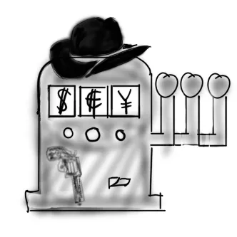
Via an industrial spy, you know how the machine works: the first arm gives $\$10$ when pulled, the second arm gives $\$1$, and the third gives $\$25$. To make the most money in the fewest pulls, which arm should we be pulling?

Yes, I agree: the optimum strategy is to pull arm $3$ every time, because it gives out the most money. That was a fairly easy one.

Now picture a different slot machine. As before, it has three arms, each with a fixed dollar value. But this time, you don’t know the values ahead of time. You want to take as few tries as possible to find the best arm, as then you can focus on pulling the best arm as often as you can. How many pulls do you need to make in total, before you know the best arm?

Now let’s apply the bandit model to your lemonade dilemma. Each arm is labelled with a possible recipe. When you pull the arm “Recipe $\mathbf{B}$”, it dispenses a cup of that lemonade, you give it to a friend to evaluate, and then you record the result ($0$ or $1$).

If there are just two arms, Recipe $\mathbf{A}$ and Recipe $\mathbf{B}$, how many arm pulls will you need to make before you know the best recipe? (Note: “best” here means “most likely to be liked by a random new friend.”)

We now have what’s called a multi-armed bandit. Each pull now has a random payout, but some arms have a higher average payout than other arms, so we want to pull those arms once we find them.

We’ll say that each recipe has some probability of success, $p$. We’re looking for the recipe with the highest probability $p$. To get an idea of the probability $p$ for a recipe, we need to take several samples.

But you’re finally in a position to see the better method! Enter Thompson sampling. Here’s the idea.

Say you give Recipe $\mathbf{A}$ to a friend, and she likes it! 🤩 How would this change the chance that, when the next friend comes along, you’ll give them Recipe $\mathbf{A}$?

Thompson sampling uses the information you gain during the test to make it more efficient while you are testing. Roughly: you serve the more promising recipes more often, but ensure that you still serve the less promising recipes occasionally, because you still want to confirm that they’re bad.

This method was first introduced in 1933, but was pretty much ignored by the academic community until decades later. Then at the beginning of the 2010’s, it was shown to have very strong practical applications which has led to a widespread adoption of the method.

The idea can be complicated to understand, but simple to implement and incredibly powerful. You’ll impress your friends with the perfect glass of lemonade.

Patience! First, you must understand a couple of probability distributions!

In your earlier A/B test, you flipped a coin to determine which page to serve a visitor. In English, you might say “Either the coin lands $\text{Heads}$ or $\text{Tails}$. It’s an unfair coin, where the probability is $60\%$ that it lands $\text{Heads}$. I flip the coin, and call its result $C$.” Here’s how you might sketch that:

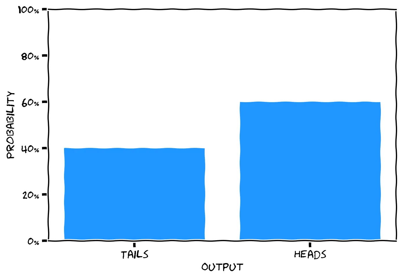
Mathematicians use a different language to say the same thing: “$C\sim \text{Bernoulli}(p=0.6)$. Therefore $P(C=1)=0.6$, and $P(C=0)=1-0.6=0.4$.”

You can read this aloud as “$C$ follows a Bernoulli distribution, with parameter $p$ equal to $0.6$. Therefore the probability that $C=1$ is $0.6$, and the probability that $C=0$ is $0.4$.” The mathematician might sketch this like so:

Now, let’s check your understanding. Say I have a biased coin that lands $\text{Tails}$ a full $70\%$ of the time. I flip the coin, and call its result $D$. How would you describe $D$?

Similarly, there is a certain underlying probability $p$ about people’s preference for a lemonade recipe. Say $R$ is the result of offering a lemonade to a random friend. They will either drink it ($R=1$) or reject it ($R=0$). In probability-speak, we can write $R\sim \text{Bernoulli}(p)$. We’re imagining each recipe is a biased coin, and trying to find the recipe with the highest $p$.

Once you have a distribution, you can generate data that fits that distribution, using sampling. To sample from the distribution below, imagine randomly picking one of the small blue squares. Once you’ve picked a random square, output the number below it.

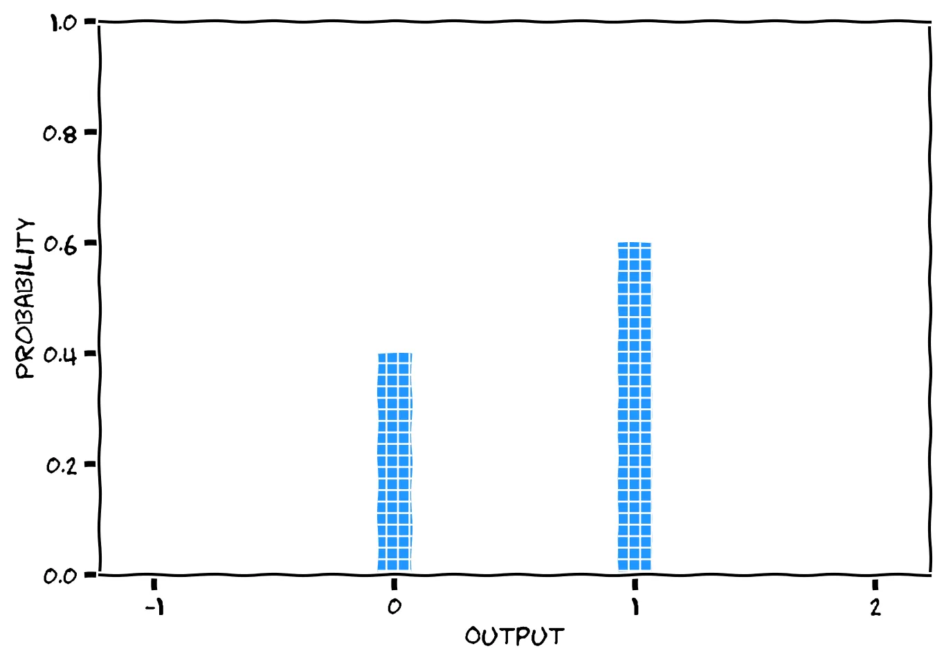
By following this procedure, you’re sampling from the distribution $\text{Bernoulli}(p=0.6)$. By doing it repeatedly, you’ll generate a list of $1$s and $0$s where $60\%$ of the results will be $1$. You can use this technique to sample from any distribution.

Indeed! Enter the Beta distribution. In a sense, the Beta distribution is the inverse of sampling from a Bernoulli distribution. It lets us go backwards: “given some samples from a Bernoulli distribution, what is its probable value of $p$?”

Let’s build some intuition. Say you make Recipe $Q$, and test it $100$ times, observing $49$ successes and $51$ failures. What do you think Recipe $Q$’s value of $p$ is?

If we sketched this intuition, we’d get something like the following:

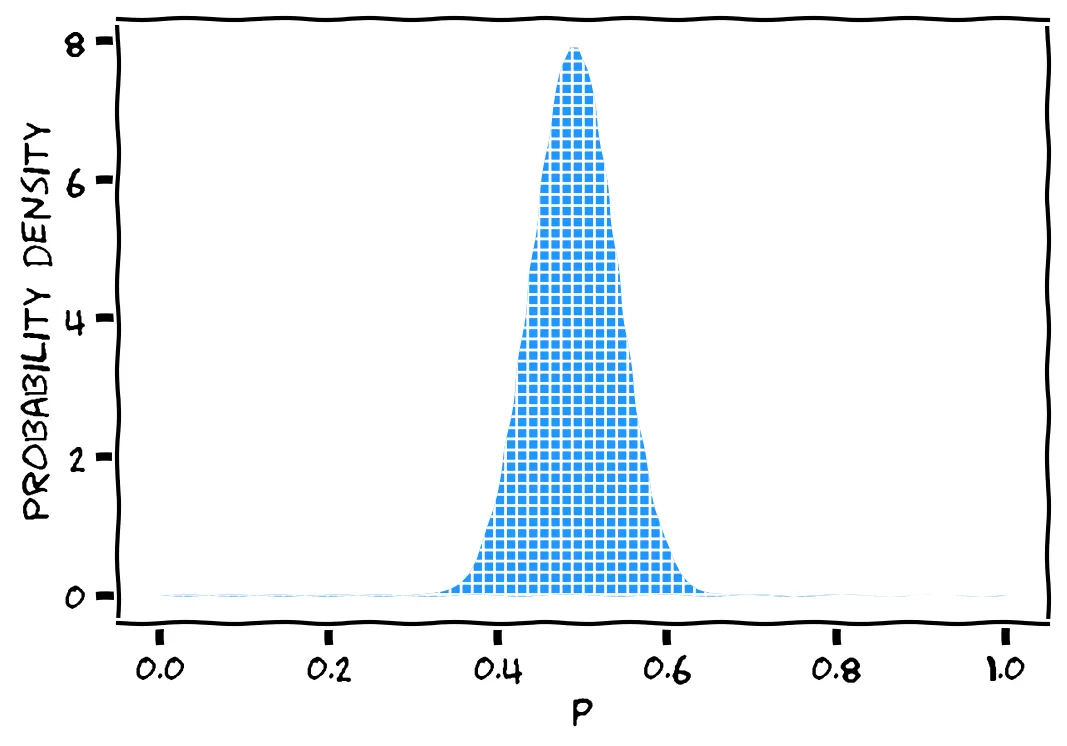
The above sketch is a probability distribution. Each small blue square is a possible value of $p$. This models our belief about $p$ after $49$ successes and $51$ failures. The value of $p$ is probably around $0.5$. It’s very unlikely to be near $0$ or $1$. But we wouldn’t be too surprised if, say, $p=0.45$.

Mathematicians call the above distribution $\text{Beta}(50,52)$. The Beta distribution has two parameters, $\alpha$ and $\beta$, which represent the number of $1$s and $0$s we’ve seen.

Well spotted! The parameters $\alpha$ and $\beta$ are the number of $1$s and $0$s we’ve seen ... plus one! So if we’ve seen $49$ successes, we should set $\alpha =50$, and if we’ve seen $51$ failures, we should set $\beta =52$.

We won’t go into the reasons for the “plus one” here. Let’s just check you understand. You encounter another one-armed bandit. When you pull its arm, it cashes out at some unknown success rate $z$. But you’ve never pulled the arm: you’ve observed zero successes and zero failures. Which distribution models your prior belief about $z$?

The sketch above is the Beta distribution’s probability distribution function, $f(x)$. You can draw it more precisely using its equation:

We won’t derive or use this equation here, but here are some example plots:

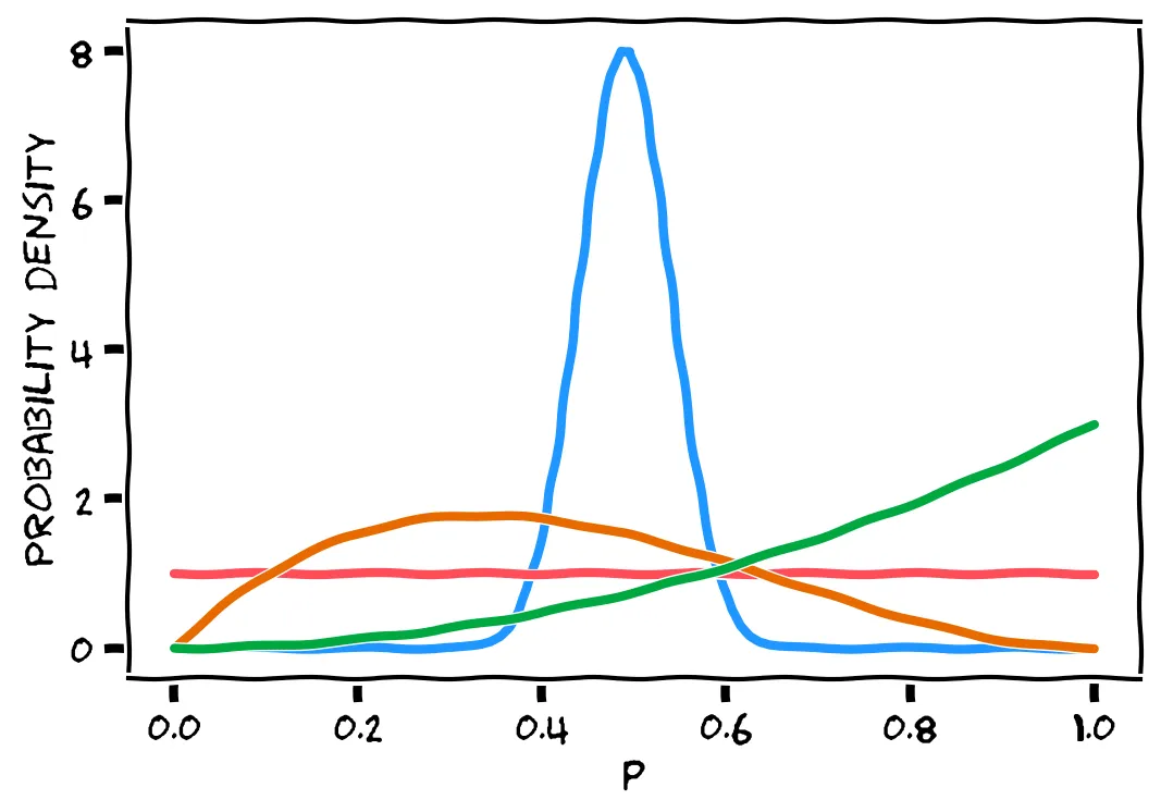
You’ve seen already that the blue line is $\text{Beta}(50,52)$. (Note, as before: you should be visualizing each line as representing all the little squares stacked under that line, each square being a possible value. But we only draw the line, so that we can draw multiple distributions in the same plot.)

There are three other lines above, and one of them is $\text{Beta}(2,3)$. But which line is it? Think about what $\text{Beta}(2,3)$ represents, and use your intuition instead of calculating.

By the way, the red line is $\text{Beta}(1,1)$, and the green line is $\text{Beta}(3,1)$. If you feel like testing yourself more, here’s a beta distribution calculator.

Okay, don’t panic: with Thompson sampling, you can test throughout the party, rather than having to do it in advance! Here’s your clipboard to tally up the results:

Recipe $\mathbf{A}$ has some success rate $a$, and Recipe $\mathbf{B}$ has some success rate $b$. We want to figure out which is highest, $a$ or $b$. We can draw their probability distribution with our current (lack of) knowledge:

Consult the plots above. What does $\text{Beta}(1,1)$ look like?

This distribution means we have no prior belief about the rates $a$ or $b$. Or, rather, we think all success rates between $0$ and $1$ are equally likely.

Oh, hi Claire! Finally we get to use the Thompson sampling algorithm! It’s a very short algorithm: guess the values of $\mathbf{a}$ and $\mathbf{b}$, then serve the recipe with the higher guess.

Guessing the value of $a$ means sampling from $\mathbf{a}$’s probability distribution. Recall the “small blue squares under the line” visualization. To make a guess, we pick a random square, then output its value on the $x$-axis.

We need to make two guesses, $g_a$ and $g_b$. Now let’s try out the algorithm on Claire.

Done! Your random sample is: $g_a=0.76$.

Done! Your random sample is: $g_b=0.63$. Now to check: do you recall what these guesses mean? When we guess that $a=0.76$, what are we really saying?

So now, which recipe should you serve to Claire?

Oh no, Claire hated it! 🤢 She takes herself to the restroom to recover, and you dutifully record her reaction on the clipboard:

Now John is arriving. No time for greetings! You need to make two new guesses. For Recipe $\mathbf{A}$, which distribution do you need to sample from?

You get two new guesses, $g_a=0.31$ and $g_b=0.59$.

... aaaand he loves it! 🤩 Once again, you record his reaction:

Let’s look at the distributions of $a$ and $b$ now:

Lucy’s about to arrive. Looking at the above distributions, which recipe are we more likely to serve her?

This doesn’t mean $\mathbf{B}$ has won yet, however! After testing out these two recipes against a few friends, you end up with:

It turns out your first two guests were anomalies! Recipe $\mathbf{A}$ is now winning. Our algorithm will now suggest lemonade $\mathbf{A}$ to our friends more often so they don’t miss out on the tastiest recipe.

As the number of wins for a lemonade gets higher, the numbers between 0 and 1 picked for that lemonade will be higher as well, making that lemonade more likely to be picked moving forward. The reverse is also true as the losses get higher, with the lemonade being less likely to get picked.

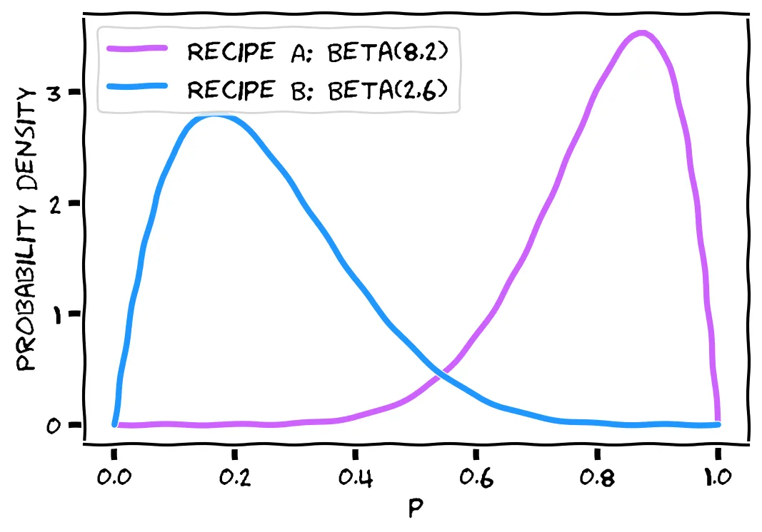
Because Thompson sampling updates itself after each new piece of information, we don’t have to wait two weeks for our results. Instead, each person we test will make the model better as we test, letting us use just our small friend group, rather than $10000$ people. It is far more efficient than the naive method we tried first, and our friends will get good lemonade much faster, resulting in less time lost drinking bad lemonade.

In the end, we have a few lines of decision-making code based on sound probabilistic principles that is guaranteed to converge. We can increase the satisfaction of our friends and quickly discover which lemonade is the best. In this case, according to our experiments, the answer is Recipe $\mathbf{A}$: 1 cup lemon juice, 1 cup sugar, and 5 cups of water. We didn’t need to test out our method against $10000$ friends to be statistically confident. And in the end, we have a foolproof method that we can apply to any number of culinary needs.