Ahh ... another lunchtime out in nature. Just you, your binoculars, and a picnic lunch. Bird-watching truly is bliss. But wait ... I hear a bird rustling under that bush! What species is it?

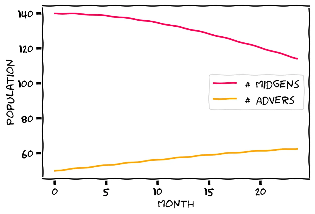
Over the past couple of years, you’ve kept diligent records on these two local bird species. Here’s the result of your tallies in chart form:

Your records are not long enough to see the long-term trends ... what you need is a kind of mathematical model to fit the data to.

However did you guess? Yes, differential equations can model all sorts of things, and are especially great when you don’t have much data (as is the case here).

So let’s start modelling the avian ecosystem from first principles: the birds and the bees. Left to themselves, Midgens beget Midgens. Those baby Midglets are adorable. 🐣 We can express this wonderful fact of life in our first Ordinary Differential Equation, or ODE:

Isn’t it fun? This is not a course in calculus, but here’s the one thing you need to know: the letter $d$ can be read as “change in”. For example, we’re using $🐦$ to stand for the number of Midgens, so $d🐦$ can be read as “change in the number of Midgens”.

Given that $t$ stands for time, what does $\frac{d🐦}{dt}$ represent?

So the equation above, in English, can be read as “The change in the number of Midgens over time is proportional to how many Midgens there are.” Here, $\alpha$ is the proportionality constant, and represents the natural growth rate of the Midgens.

This is perhaps the simplest ODE, but it’s already interesting. For example, what would happen if $\alpha =0$?

Let’s say we set $\alpha =0.002$. That is, each day, each Midgen begets $0.002$ new Midglets. Or to put it in more familiar terms, each Midgen has a baby every $500$ days.

Run this model in your head. How does the population grow over time?

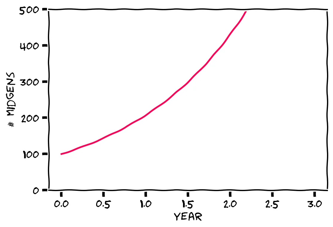
Luckily, we don’t have to run it in our head! Instead, we can run it with an “ODE solver” like scipy.integrate. Later, you’ll learn how to do this; for now, here’s the graph:

Well, look at that. Exponential growth! Without any competition, the Midgens will multiply unchecked.

Indeed. This is not an accurate model. So far you’ve learned how to model change in one variable (🐦), but the world is more complex. Let’s learn how to deal with a second variable: the number of Advers (🦅).

The Midgens are a prey species, kept in check by the predator Advers. They eat those innocent Midglets. 🍳 We must add this second fact of life to our mathematical model. Here’s the full model, called the predator-prey model:

You can interpret this with some thought.

The term $🐦🦅$ is the number of Midgens multiplied by the number of Advers. You can think of this as the number of interactions between the two species. $\beta$ says how frequently those interactions result in a dead Midgen, and $\delta$ says how much those dead Midgens are converted into new Advers.

Now, think about the term $-\gamma 🦅$. It’s used in the second equation, describing the change in Advers over time ($\frac{d🦅}{dt}=\dots -\gamma 🦅$). What could that term $-\gamma 🦅$ represent?

To actually use this model, you need to estimate these parameters. But luckily, you have also studied the birth, death, and kill rates, and you use these to come up with:

(Note that $\gamma$ is positive! A population of Advers on their own will die off, rather than grow.)

Now, try again to run this model in your head. It’s pretty difficult, isn’t it?

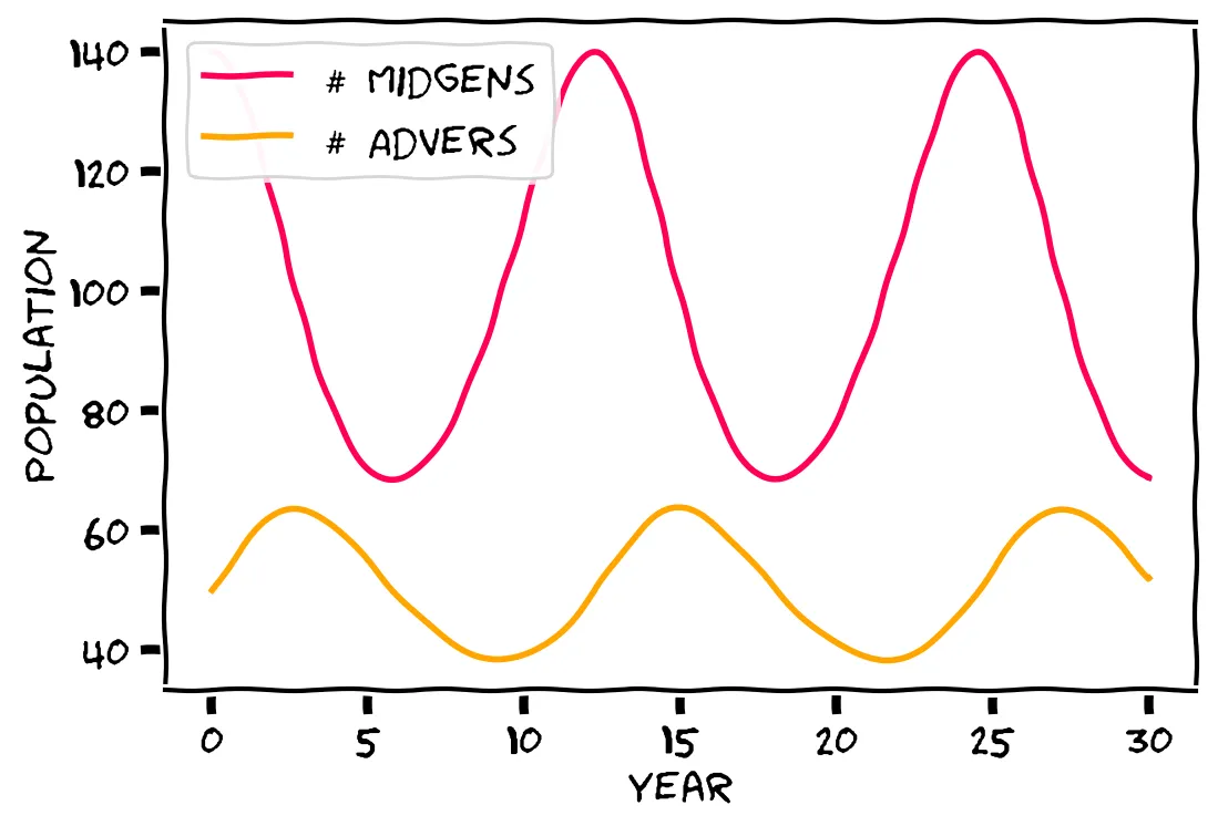
Okay, here’s your graph:

The population change is cyclical! You’ve now seen two kinds of system: one that never reaches a stable state, and another that reaches a kind of cyclic stability.

Finally, your observations make sense. You saw a dip in the Midgen group and a growth in the Advers, but soon the trends will reverse again: the Advers will become victims of their own success, destroying their food supply and killing each other. The circle of life continues.

Oh yes! We can translate a model into Python by defining an initial state, and a function that describes the rate of change. Here’s a Python equivalent of our first model, which grows exponentially:

We can then use the scipy.integrate package to run this model:

Finally, we can graph the timeline with:

That’s basically all the Python you need to know! For the complete runnable code, check out our Colab notebook.

And now for something completely different. You’ve learned the basics of ODEs and how to run them. Now you’ll use them to model a very real-world complex system: your own body! 🚶‍♀️

Last year, my bathroom scales said I weighed $55$ kg. A ruler says I am 1.82 meters tall. This put my BMI at $17$, which is classified as underweight. I set myself the target of reaching at least $63$ kg, bringing my BMI into the “healthy” range. But how could I achieve this?

We’ve all been told: If you eat more calories than you burn, you will ...

And this advice is basically true, but makes it sound simple. We often talk about the $2000$ kcal diet as if it were a universal truth, but each person is different! How many calories are you burning right now?

Again, you need a model. Given a target weight, you can calculate your personal caloric intake using a ‘weight change’ ODE.

We’ll call the amount you intake $\mathbf{EI}$, and the amount you expend $\mathbf{EE}$. The difference $\mathbf{EB}=\mathbf{EI}-\mathbf{EE}$ is called your energy balance. If your intake equals your expenditure, $\mathbf{EB}=0$, you’re perfectly balanced, and your weight will be stable.

We’ll measure all of these in kilocalories (usually just pronounced “calories”) per day. Yesterday, I ate $2500$ kcal, and I burned $2700$ kcal. What was my energy balance for the day?

So these variables are measurements of energy, but ultimately we’re concerned with weight. How are energy and weight related? Einstein had important opinions here ⚛️, but instead we’ll use a model developed by Gilbert Forbes. Forbes says, if you squint, your body (measured in kg) is made up of two kinds of tissue :

Now, check the nutritional fact label 🏷️ on the back of your neck:

It’s been there since birth! (Your figures might differ a little bit from the Forbes model, but probably not by much.)

This label is helpful alongside a modern bathroom scale, which reports weight and percentage fat. Let’s try that out. Kevin’s scale says he weighs $110$ kg, of which $10$ kg is fat. What is Kevin’s total calorific content?

(Incidentally, this means you could use Kevin to heat one liter of water to around $274000°\text{C}$. But just because you could, doesn’t mean you should.)

Now, when you eat, should your body build more Fat tissue or more Lean tissue? We call your body’s decision $p$: it’s a proportion between $0$ and $1$. If $p=0$, your body only builds/burns Fatty tissue. If $p=1$, your body only changes Lean tissue.

But how does your body make this decision, $p$? Forbes says it’s based on how much fat you have. The model looks like this:

$C=54.3$ is a magic constant. Let’s sanity-check this function. Say you have no fat on you, and then you eat a meal. Does your body use the meal to build Fat tissue or Lean tissue?

On the other hand, as $\text{Fat}$ tends to $\infty$, your body only burns/builds Fat tissue.

We can now write two ODEs describing how your body changes:

Here, your net energy $\mathbf{EB}$ is being shared between your Lean and Fat tissue, and then converted from kcal to kg.

Now recall the original equation, $\mathbf{EB}=\mathbf{EI}-\mathbf{EE}$. The value $\mathbf{EI}$ is just how much we decide to eat, and we will play with $\mathbf{EI}$ to obtain our target output weight.

But calculating the energy expenditure $\mathbf{EE}$ is more complicated. Let’s simplify the problem by assuming that you never move.

No, you can keep your shape. Bed-bound, your body burns fuel just to stay alive. This is called your basal metabolic rate, or $\mathbf{BMR}$, measured in kcal per day. Here is Forbes’ model:

Don’t panic! 🙂 The first line here just says it takes energy to maintain current tissue. The second line says it takes energy to build new tissue.

Now just consider the last term, $\mathbf{BMR}=\dots +0.14\mathbf{EI}$. How would you interpret this term?

Yes, it even takes energy to consume energy! (This is called the Thermic Effect of Food.)

Now you should understand why bears store fat when hibernating: to store the same energy as lean tissue, they would need five times as much space! And to maintain that lean tissue would cost almost seven times as much! 🐻‍❄️

Finally, to get your energy expenditure $\mathbf{EE}$, Forbes says you must multiply your basal metabolic rate by your physical activity level, called $A$. Now, how many hours do you exercise per day?

The activity level is an abstract number between $1.4$ (no exercise) and $2.4$ (multiple hours of exercise every day).

Note that “no exercise” is still above $1$: you probably move around more than what’s considered truly “basal”.

Note also that exercise is not just added to your metabolic work — it multiplies your metabolic work! By exercising, you make your body spend more even when it’s resting!

Finally, we solve for the energy balance $\mathbf{EB}$. I’ll spare you the algebra! Here’s the ugly but functional equation:

We now have everything we need to run the model. But again, try to run the model in your head first! For example, given a high-calorie diet like $\mathbf{EI}=4000$ kcal, my weight will start increasing, but what will happen to my weight eventually?

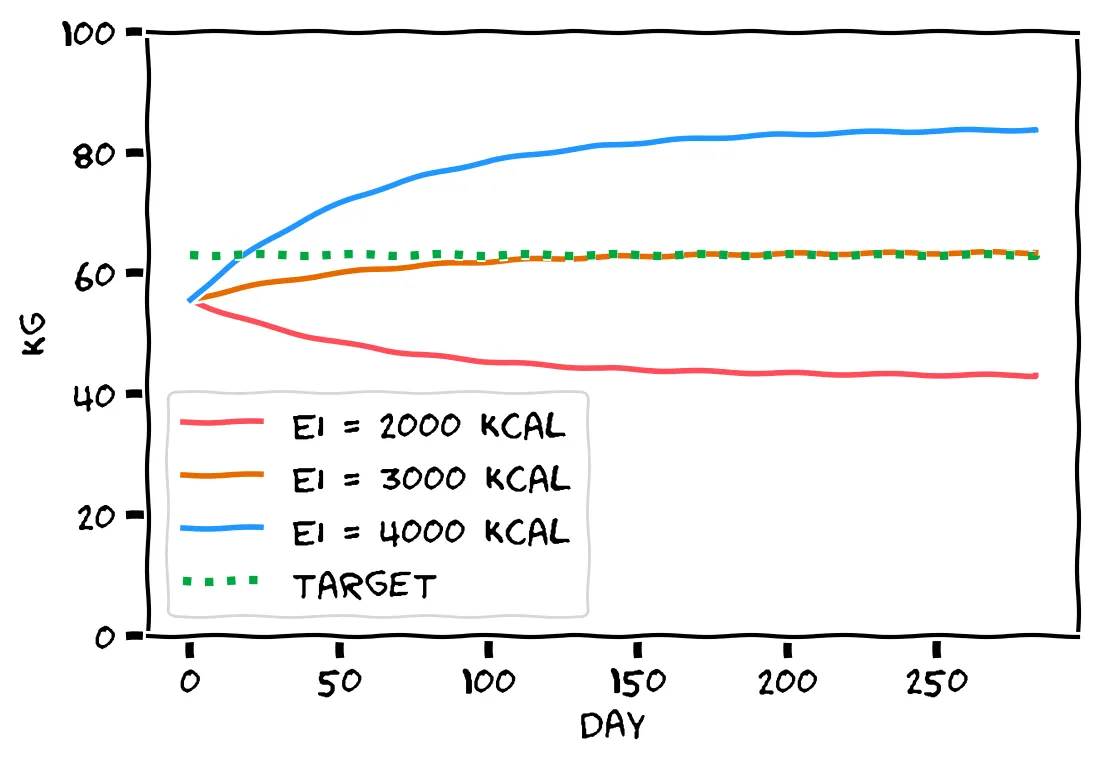
Well, let’s find out! Using the trusty ODE solver, here are various plots with different values of $\mathbf{EI}$:

It turns out that weight always approaches a stable state! My personal goal is to reach $63$ kg. How much should I consume per day?

I was able to follow this regimen (although it was quite challenging) and move much closer to a healthy weight. It takes a lot of effort to maintain your health, but by using all of the tools at your disposal, you can give yourself the best chance to meet your goals.

You’ve now seen three types of system: one system with no stable state, one system with cyclic behavior, and one system that settles to a stable state. Differential equations are very expressive!

End notes:

For the complete runnable code, check out our Colab notebook.

The predator-prey model was originally designed by Lotka and Volterra.

They’re called ordinary differential equations because we only talk about change with respect to time. Or, more precisely, a single independent variable, which in all our models was the time $t$.

Roughly speaking, odeint just repeatedly runs our rate_of_change function, and sums up the outputs. Although it does clever stuff to be more accurate and efficient. You could look into Runge-Kutta methods.

For more details on the weight model, peruse “Modeling weight-loss maintenance to help prevent body weight regain” or “Quantification of the effect of energy imbalance on bodyweight”.